Demo 1: Prediction of Multiple Correlated Tasks with Individual Training Data
File name: demoMTGP.m
This is the first example which illustrates the differences between regression tasks using normal GPs and MTGPs. To use demoMTGP.m, please include the path of the GPML toolbox or specify the path in demoMTGP.m (line 6). The example contains 5 cases. The first case is the simplest case, which will be sequentially extended by each following case by certain aspects. Please select one of the cases using the variable MTGP_case (line 24).
line 24:MTGP_case = 1% default method
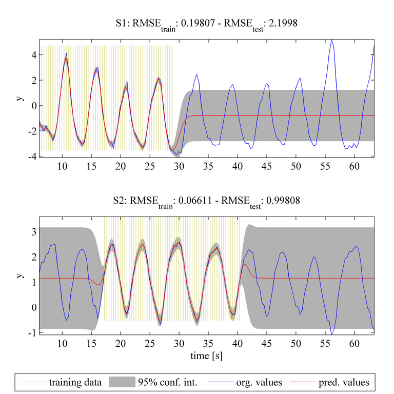
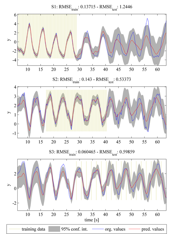
The plots above show the original "ground truth" dataset (blue solid line) for two periodical tasks (S1 and S2). The shaded yellow regions indicate the known training data for each task. For example, in the upper plot, we assume that data in the region t < 28 are available as training data. The results are generated by the MTGP toolbox using a squared exponential temporal covariance function K_t, assuming that the tasks are independent of each other. The hyperparameters of the covariance function were not optimised. The prediction values are shown with a red solid line (for the mean function) and the 95% confidence interval with the shaded grey area. The root mean square error (RMSE) of the predictions compared with the training and test data for each task is shown above the plots.
The predictions shown in the two plots above can be interpreted as being those from using a single-task GP model on each time-series independently (in which correlation between tasks is not considered). Even though the tasks have different known training datasets, the prediction for the test data of each task is mainly the mean of the training data, as independence between the tasks is assumed.
line 24:MTGP_case = 2
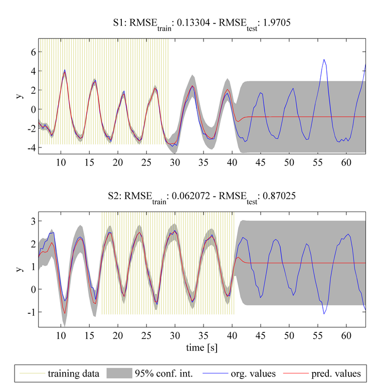
This case is an extension of case 1 using the same tasks, training data, and covariance function as before. However, in contrast to case 1, the MTGP model is initialised assuming independence between the tasks and then the hyperparameters of the GP are optimised by minimising the negative log marginal likelihood (NLML). The plots above again show the original dataset with the blue line, the training data as the shaded yellow region, and the predicted values as a red solid line and with the 95% confidence interval as shaded gray area. Compared to case 1, the MTGP model learns the negative correlation that exists between the tasks. This information improves the predicted results for task S1 (shown in the upper plot) in the range of t = [30 40]s. Similarly, improved predictions may be seen for task S2 (shown in the lower plot) in the range t = [0 15]s. We can see that there is also a decrease in RMSE_test for both tasks, when compared with the RMSE_test values from case 1.
line 24:MTGP_case = 3
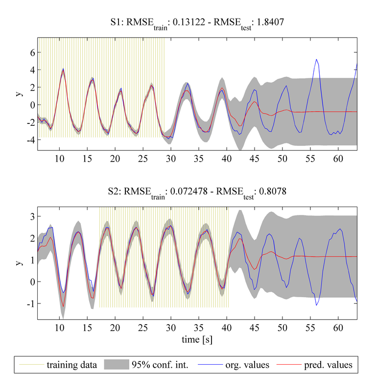
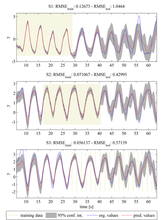
MTGP models can be extended to an arbitrary number of tasks. Assuming that a third task S3 is given, the task can be easily integrated into the MTGP model. We note that task S3 has a different sampling frequency - the MTGP model can cope with tasks of differing sampling frequencies in a straightforward manner. Similar to cases 2 and 3, considered previously, the model is here initialised assuming that all tasks are independent of each other. By optimising the NLML again, the MTGP model learns the correlation between tasks. We can see that inclusion of task S3 results in a further improvement in the prediction accuracies of tasks S1 and S2, with further decreases in RMSE_test compared with that from previous cases.
line 24:MTGP_case = 5
The final case in demo 1 illustrates how MTGP models can be extended to model task-specific noise. (In all previous cases, the noise was assumed to be the same for each task.) To show this, an additional noise component has been added to the original data from task S2. The temporal covariance function is now extended from a quasi-periodic function to a sum of a quasi-periodic and a noise covariance function. The noise covariance function adds one hyperparameter for each task expressing the noise for each task. The console displays the values of the hyperparameters learned for these GPs, and, as expected, it may be seen that the second hyperparameter, corresponding to the noise of task S2, takes a higher value compared with those for tasks S1 and S3.

- Research
- SonoBox: A Robotic Ultrasound System for Pediatric Forearm Fracture Diagnosis
- Robotics Laboratory (RobLab)
- OLRIM
- MIRANA
- Robotik auf der digitalen Weide
- KRIBL
- Ultrasound Guided Radiation Therapy
- Digitaler Superzwilling: Projekt TWIN-WIN
- - Finished Projects -
- High-Accuracy Head Tracking
- Neurological Modelling
- Modelling of Cardiac Motion
- Motion Compensation in Radiotherapy
- Navigation and Visualisation in Endovascular Aortic Repair (Nav EVAR)
- Autonome Elektrofahrzeuge als urbane Lieferanten
- Goal-based Open ended Autonomous Learning
- Transcranial Electrical Stimulation
- Treatment Planning
- Transcranial Magnetic Stimulation
- Navigation in Liver Surgery
- Stereotactic Micronavigation
- Surgical Microscope
- Interactive C-Arm
- OCT-based Neuro-Imaging