Demo 3: Tasks with Different Temporal Characteristics
File name: demoMTGP_convoluted_kernels.m
So far, it has been assumed that all tasks share similar temporal characteristics (e.g., that periodicity and noise can be described by the same covariance function for each task). This demo illustrates how the MTGP framework can cope with tasks that have different characteristics (in case 1) and shows how MTGP models can be further modified to allow task-specific temporal characteristics (in case 2). This is achieved using convoluted kernels. To use demoMTGP_convoluted_kernels.m, please include the path of the GPML toolbox or specify the path in demoMTGP_convoluted_kernels.m (line 9). The example contains 2 cases. Please select one of the cases by specifying the variable MTGP_case (line 22).
line 22:MTGP_case = 1% default method
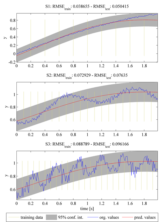
The plots above show the original dataset (shown by the blue solid line) of three tasks (S1 - S3). Tasks S2 and S3 were generated by adding an additional sinusoidal component (with a small amplitude and with Gaussian noise) to task S1. Each task is sampled at a different frequency (marked by the vertical yellow lines). The predictions were generated by the MTGP toolbox using a squared exponential temporal covariance function k_t. The model was initialised assuming perfectly-correlated tasks. The predictions are shown by the red solid line and the 95% confidence interval is shown by the shaded grey area. In this case, each task is constrained to share the same values for their respective hyperparameters, and it may be seen that the predictions provided by the the MTGP model are a compromise over all tasks. The smaller variations in the amplitude of task S2 and S3 cannot be modelled, and it may be seen that the dynamics of task S1 are dominating.
line 22:MTGP_case = 2

If the variations in the amplitude of tasks S2 and S3 are to be modelled within a single model, the MTGP can be extended by using task-specific hyperparameters. This is possible by using a convolution of covariance functions. The figures show the predictions for the tasks presented in case 1. Now, however, each task has a task-specific covariance hyperparameter. It may be observed that each task can be modelled more precisely. The values of the optimised hyperparameters representing the temporal scaling are 1.45, 0.47, 0.08 for tasks S1, S2, and S3, respectively. As expected, this time-scale parameter decreases as the dynamics of the task become more rapidly-changing.

- Forschung
- SonoBox: Ein Roboter-Ultraschallsystem zur Diagnose von Unterarmfrakturen bei Kindern
- Robotics Laboratory (RobLab)
- OLRIM
- MIRANA
- Robotik auf der digitalen Weide
- KRIBL
- Ultraschallgeführte Strahlenchirurgie
- Digitaler Superzwilling: Projekt TWIN-WIN
- - Abgeschlossene Projekte -
- Hochpräzise Bewegungsverfolgung am Kopf in der Strahlentherapie
- Neurologische Modellierungen
- Modellierung von Herzbewegungen
- Bewegungskompensation in der Strahlentherapie
- Navigation and Visualisation in Endovascular Aortic Repair (Nav EVAR)
- Autonome Elektrofahrzeuge als urbane Lieferanten
- Ziel-basierendes lebenslanges autonomes Lernen
- Transkranielle Elektrostimulation
- Bestrahlungsplanung
- Transkranielle Magnetstimulation
- Navigation in der Leberchirurgie
- Stereotaktische Mikronavigation
- OP - Mikroskop
- Interaktiver C-Arm
- OCT-basierte Neurobildgebung